Learning Objectives
By the end of this study guide, the learner should be able to:
- Explain the basic principle of pulsed radar operation and distinguish between monostatic and bistatic configurations.
- Derive the radar range equation step by step from first principles (power density, antenna gain, RCS and free-space spreading).
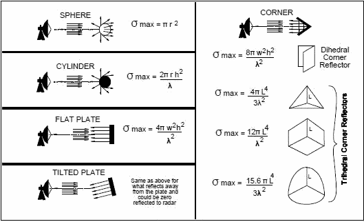
- Define and compute the radar cross section (RCS, σ) of simple targets such as spheres, cylinders and flat plates.
- Account for receiver noise, noise figure and minimum detectable signal (MDS) in radar range prediction.
- Calculate the maximum detection range of a radar and analyse its sensitivity to peak power, antenna gain, wavelength and RCS.
- Evaluate radar performance limitations: pulse repetition frequency (PRF), unambiguous range, blind speeds, eclipsing and atmospheric attenuation.
- Use interactive simulations to verify the radar range equation and PRF constraints.
1. Introduction: The Basic Radar Principle
Radar (Radio Detection and Ranging) is an electromagnetic system used to detect the presence of, and determine the location and velocity of, distant objects (targets). It does so by transmitting electromagnetic energy and processing the echo returned from the target. The distance follows from the measured round-trip delay:
1.1 The Monostatic Radar
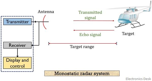
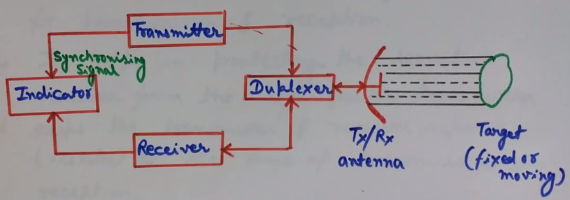
In a monostatic radar, a single antenna (shared through a duplexer) is used for both transmission and reception. This is the most common configuration, used in ground stations, weather radar and many satellite tracking systems.
1.2 The Bistatic Radar
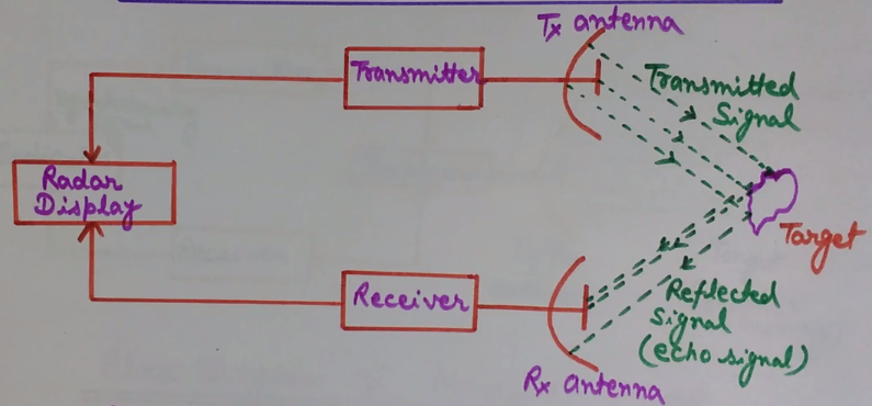
In a bistatic radar, the transmitter and receiver are separated by a distance comparable to or greater than the target range. Bistatic geometries are useful in satellite links, passive radar and stealth detection, because the receiver is located away from the transmitter and does not itself radiate.
2. Derivation of the Radar Range Equation
The radar range equation relates the received echo power to the transmitted power, antenna parameters, target properties and range. Derive it in four steps.
2.1 Solving for Maximum Range
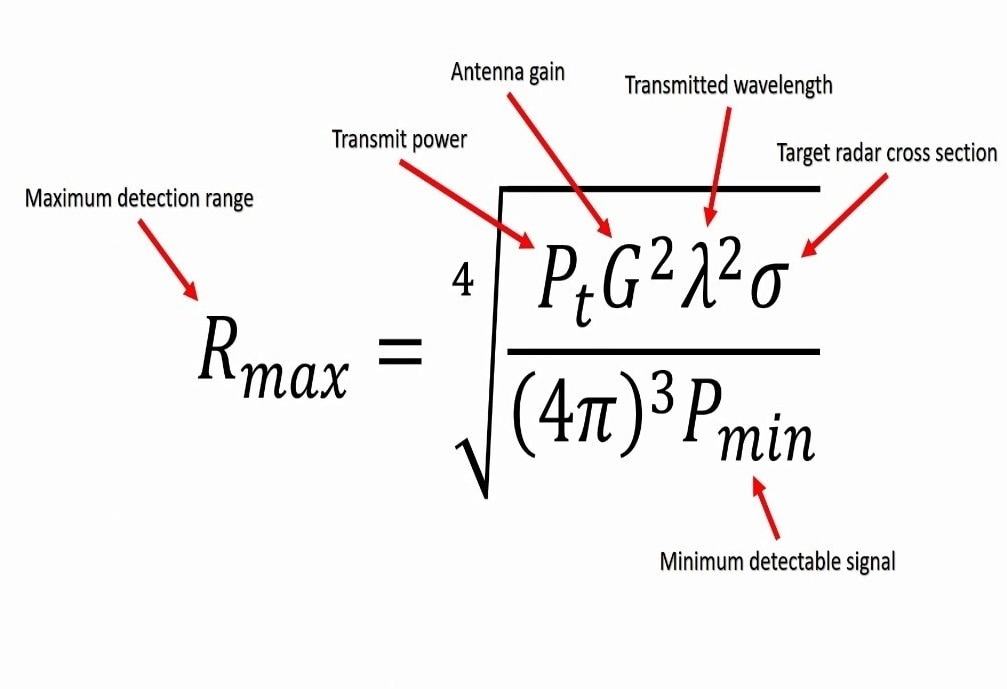
Setting Pr equal to the minimum detectable signal Smin (see Section 4) and solving for R gives the maximum detection range:
Useful dB form (powers in dBW, G and σ in dB):
2.2 Practical (Modified) Range Equation
Real systems include system losses L (feeds, duplexer, atmospheric absorption, beam shape, integration loss) and a pattern propagation factor F:
2.3 Search and Tracking Forms
- Search radar: power is spread over a large solid angle Ω. The range equation becomes Pr = PavAeσ/(4πΩR4) — showing that for a fixed search duty, average power and antenna aperture (not peak power alone) drive range.
- Tracking radar: energy is concentrated on a single target, using the standard equation with dwell-time integration gains.
3. Radar Cross Section (σ)
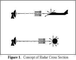
The radar cross section of a target is the (fictitious) area that would intercept an amount of incident power which, if scattered isotropically, would produce the observed echo power back at the radar:
σ depends on the target's physical size, shape, material, frequency and aspect angle — it is not simply the physical area.
| Target | Typical RCS | Comment |
|---|---|---|
| Insect / bird | 10−5 – 10−2 m² | Rayleigh region (a << λ) |
| Small UAV / missile | 0.01 – 0.5 m² | Stealth shaping reduces this |
| Fighter aircraft | 1 – 10 m² | Highly aspect-dependent |
| Large airliner | 10 – 100 m² | Optical region |
| Ship | 103 – 105 m² | Superstructure dominates |
| Sphere (radius a, a >> λ) | σ = πa2 | Equals its projected physical area |
4. Receiver Noise, Noise Figure and Minimum Detectable Signal
The weakest echo a radar can detect is set not by the transmitted power but by noise. The dominant noise source is thermal (Johnson–Nyquist) noise from the receiver front end.
4.1 Thermal Noise Power
At T0 = 290 K, the noise spectral density is kT0 = −174 dBm/Hz. For a 1 MHz bandwidth, N ≈ −114 dBm.
4.2 Noise Figure and Noise Temperature
The receiver degrades the signal-to-noise ratio by its noise figure F (or equivalent noise temperature Te = (F−1)T0):
The total input-referred noise is Ni = kT0BnF. For cascaded stages, use Friis' formula: F = F1 + (F2−1)/G1 + (F3−1)/(G1G2) + ... which is why the first amplifier (LNA) at the antenna must have the lowest possible noise figure.
4.3 Minimum Detectable Signal
The minimum detectable signal (MDS), also called the minimum discernible signal, is the received power for which the output SNR just equals the detectability threshold (SNR)1 required by the detector (typically 10–16 dB, and lower with pulse integration):
Substituting into the range equation:
5. Factors Affecting Radar Performance
5.1 Pulse Repetition Frequency and Unambiguous Range
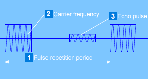
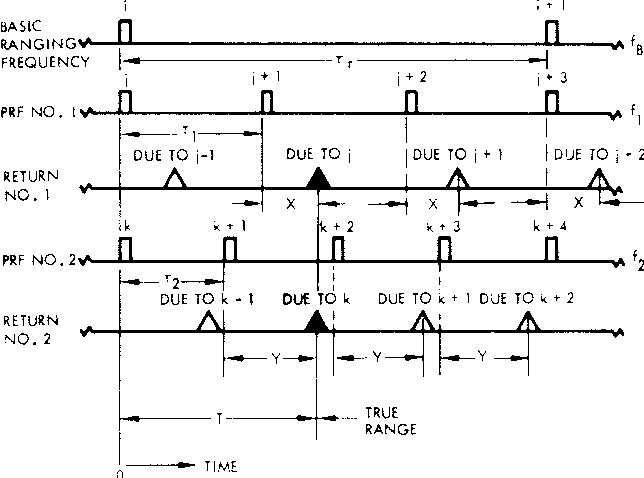
A pulsed radar transmits pulses at a rate called the pulse repetition frequency (PRF). The echo from a distant target must return before the next pulse is transmitted, otherwise the measured delay is ambiguous. The maximum unambiguous range is:
Low PRF (long unambiguous range) suits range measurement and ground mapping; high PRF suits Doppler/velocity measurement but folds ranges. Medium PRF is a compromise.
5.2 Doppler Frequency and Blind Speeds
A target with radial velocity vr produces a Doppler shift fd = 2vr/λ. The PRF also determines the unambiguous Doppler interval (=±PRF/2). Moving-target-indicator (MTI) radars cancel stationary clutter using delay-line cancelers, but targets at blind speeds vb = n·λ·PRF/2 (n = 1, 2, ...) produce zero Doppler after cancellation and are lost.
5.3 Eclipsing and Minimum Range
During the transmitted pulse (width τ), the receiver is blanked; targets closer than Rmin = cτ/2 return echoes that arrive while the radar is still transmitting and are eclipsed. Short pulses improve range resolution (ΔR = cτ/2) but reduce average power.
5.4 Atmospheric Attenuation and Propagation
At radar frequencies, absorption by oxygen and water vapour (peaks near 22 and 60 GHz), rain, and multipath/ducting all reduce performance. The two-way atmospheric loss must be included as a term in L of the modified range equation. This is especially important for satellite-earth paths traversing the whole atmosphere.
5.5 Summary of Performance Trade-offs
| Parameter ↑ | Effect on range/performance |
|---|---|
| Peak power Pt | ↑ range (fourth-root law); limited by hardware |
| Antenna gain G | Very strong effect (G appears squared) |
| Wavelength λ | Longer λ → more received power, but larger antenna for same gain |
| Target RCS σ | Larger σ → longer detection range |
| Bandwidth Bn | ↑ B → ↑ noise → ↓ range (but better resolution) |
| Noise figure F | ↑ F → ↓ range |
| PRF | Sets unambiguous range and Doppler window |
6. Animation: Two-Way Radar Propagation & the R−4 Law
Watch a pulse travel from the radar to the target and back. The echo amplitude bar shows how rapidly the returned power falls with range — the physical origin of the 1/R4 dependence in the radar equation.
7. Interactive Simulations
Simulation 7.1 — Radar Range Equation Calculator
Vary the system parameters and observe the received power, SNR and maximum detection range. Use it to verify the worked examples and explore sensitivity (the fourth-root law).
Received SNR vs. Range
Simulation 7.2 — PRF, Unambiguous Range and Blind Speeds
Explore the fundamental PRF trade-off: low PRF gives long unambiguous range; high PRF pushes blind speeds up and widens the unambiguous Doppler window.
8. Self-Check Questions
Attempt each question, then click to reveal the answer.
Q1. Why does the received power vary as 1/R4 rather than 1/R2?
Q2. A radar's peak power is increased 16×. By what factor does the maximum range increase (all else constant)?
Q3. Compute the noise power in dBm for Bn = 2 MHz and F = 3 dB.
Q4. What is the maximum unambiguous range for PRF = 2 kHz?
Q5. A 3 GHz radar uses PRF = 1 kHz. Find the first blind speed.
Q6. Explain why the LNA noise figure dominates overall receiver noise figure.
Q7. A sphere of radius 0.5 m operates in the optical region at 10 GHz. Estimate its RCS.
Q8. How does atmospheric absorption affect the radar equation for a satellite ground station?
9. References and Further Reading
- M. I. Skolnik, Introduction to Radar Systems, 3rd ed., McGraw-Hill, 2001 (Chapter 2: The Radar Equation).
- M. I. Skolnik (ed.), Radar Handbook, 3rd ed., McGraw-Hill, 2008.
- C. A. Balanis, Antenna Theory: Analysis and Design, 4th ed., Wiley, 2016 (effective aperture and gain relations).
- G. W. Stimson, Introduction to Airborne Radar, 2nd ed., SciTech, 1998.
- Agilent / Keysight Application Note 150-9, Radar Measurements.
- Electronics Desk, “Radar System — Definition, Block Diagram”, electronicsdesk.com.
- RF Cafe, EW & Radar Systems Engineering Handbook — Radar Cross Section, rfcafe.com.