EEEN 567 - Satellite Engineering | Study Guide: CW Radar & FMCW Radar

Learning Objectives

By the end of this study guide, the learner should be able to:

Explain the operating principle of a continuous-wave (CW) radar and draw its block diagram.
Derive the Doppler frequency shift f_d = 2v_r/λ for a moving target and use it to measure radial velocity.
State the CW radar range equation and explain why an unmodulated CW radar cannot measure range.
Explain the single-frequency CW limitation and the role of IF amplification and sideband filtering in practical CW Doppler radars.
Describe the FMCW radar waveform (linear frequency sweep / chirp), its block diagram, and the generation of the beat frequency.
Derive and apply the FMCW ranging relations R = c·f_b·T_c/(2B) and the up-chirp/down-chirp method for simultaneous range and Doppler (velocity) measurement.
Identify applications of CW and FMCW radar, including radar altimeters used in satellite and aircraft systems, police speed guns, and automotive radars.
Use the interactive animations and simulations to verify Doppler and FMCW beat-frequency calculations.

1. Introduction to Continuous-Wave (CW) Radar

A continuous-wave radar transmits an unmodulated (constant-frequency, constant-amplitude) sinusoid continuously — there are no pulses. Reception takes place simultaneously with transmission (separate transmit/receive antennas, or a circulator/isolator). Because there is no time reference marking transmission instants, a simple CW radar cannot measure range. What it measures extremely well is radial velocity, through the Doppler frequency shift of the echo.

Key contrast with pulsed radar: pulsed radar measures range from echo delay; unmodulated CW radar measures velocity from echo frequency shift. To get range with a CW waveform, the carrier must be frequency-modulated — that is the FMCW radar of Section 4.

1.1 CW Radar Block Diagram

The transmitted signal leaks into the receiver, where it is mixed with the Doppler-shifted echo. The mixer output contains a component at the Doppler difference frequency f_d, which is filtered, amplified and measured with a frequency counter.

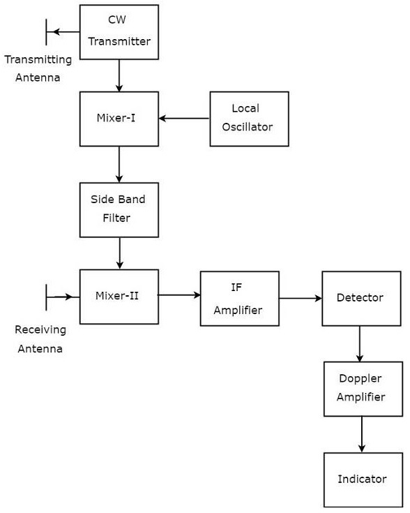
1.2 CW Radar with IF Amplification

In practical systems the Doppler frequency can be too low for stable amplification, so the received signal is first translated to a convenient intermediate frequency (IF) using an IF oscillator. The Doppler information rides on the IF as sidebands (f_IF ± f_d).

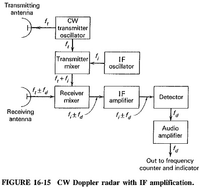
Fig. 2 — CW Doppler radar with IF amplification (textbook Fig. 16-15). The Doppler shift f_d appears after detection and is counted.

1.3 Advantages and Limitations of CW Radar

Advantages	Limitations
Simple, low-cost hardware (no high-power pulser)	Cannot measure range without modulation
Continuous illumination → high average power on target	Transmit leakage into receiver can mask weak echoes
Excellent velocity accuracy and sensitivity (Hz-class Doppler)	Radial velocity only; no direction of motion sign without IQ processing
No minimum-range (eclipsing) problem	Stationary clutter competes directly with the Doppler signal

2. The Doppler Effect in Radar

When a target moves with radial velocity v_r (positive = approaching), the round-trip path shortens or lengthens while the wave is in flight. Each successive transmitted cycle travels a slightly different distance, so the echo frequency differs from the transmitted frequency by the Doppler shift:

f_d = 2v_r / λ = 2v_rf_c/c The factor 2 arises because the path changes twice per wavelength (two-way travel). Approaching target: echo frequency increases (f_c + f_d); receding: decreases (f_c − f_d).

2.1 Worked Example

Example 2.1: A 9.5 GHz (X-band) police radar measures a Doppler shift of 1.58 kHz from an approaching vehicle. What is its speed?

λ = c/f = 3×10⁸/9.5×10⁹ = 0.0316 m. v_r = f_dλ/2 = 1580 × 0.0316/2 = 25 m/s = 90 km/h.

2.2 Sign of the Doppler — Direction of Motion

A simple envelope detector loses the sign of f_d (approach vs. recede look identical). Practical CW radars therefore use in-phase/quadrature (I/Q) demodulation: two mixers driven by local-oscillator signals 90° apart preserve the sign of the Doppler frequency, giving unambiguous direction of motion.

3. The CW Radar Range Equation

Because the CW waveform is a single spectral line, the radar equation takes the same form as for pulsed radar (average power replaces peak power):

P_r = P_tG²λ²σ / [(4π)³R⁴L]

where P_t is the continuous transmit power, G the common antenna gain (monostatic), σ the RCS, R the range and L the system losses. The Doppler signal power delivered to the Doppler amplifier is P_r/2 (half the power sits in the image sideband that filtering removes).

Design insight: since the Doppler shift can be measured to fractions of a Hz with long observation times, CW radars achieve extraordinary velocity resolution. However, the 1/R⁴ dependence still applies, and the transmitter-to-receiver leakage must be kept below the expected echo level through antenna isolation (typically 80–120 dB) and, in FM-CW altimeters, through careful sidelobe design.

4. Frequency-Modulated CW (FMCW) Radar

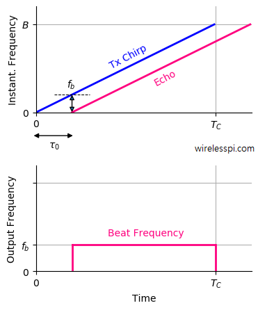
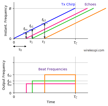
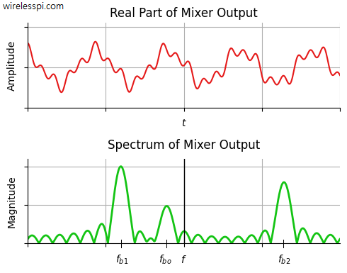
An FMCW radar transmits a continuous wave whose frequency is swept linearly in time (a chirp), typically as a sawtooth or triangular waveform. The echo from a target at range R is a delayed replica of the transmitted chirp. Mixing the received echo with the currently-transmitted signal produces a constant-frequency difference called the beat frequency f_b, which is directly proportional to range.

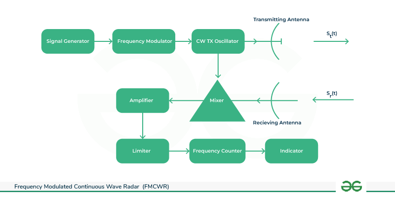
Fig. 3 — FMCW radar block diagram: signal generator, frequency modulator, CW oscillator, antennas, mixer, amplifier/limiter, frequency counter and indicator.

FMCW chirp and beat frequency — Fig. 4 — FMCW principle: the echo chirp is a delayed copy of the transmitted chirp; their constant frequency offset during the sweep is the beat frequency f_b.

4.1 Block Diagram of a Modern FMCW Transceiver

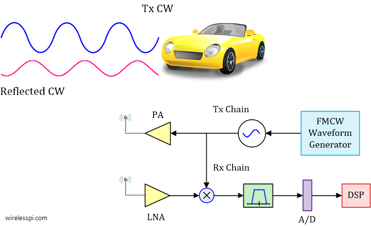
In digital FMCW systems the beat signal is digitised and processed with an FFT; each target appears as a spectral peak at its beat frequency, giving a range profile.

FMCW multiple targets — Fig. 6 — Multiple targets produce different delays τ₁, τ₂ … hence different beat frequencies fᵡ₁, fᵡ₂.

FMCW mixer output and FFT — Fig. 7 — Mixer output time waveform and its spectrum: beat notes at fᵡ₁, fᵡ₂ are resolved by the FFT, and fᵡ₀ can indicate clutter.

5. FMCW Range and Doppler Measurement

Consider a linear up-chirp sweeping bandwidth B in chirp duration T_c. The chirp slope is μ = B/T_c (Hz/s). A target at range R returns an echo delayed by τ = 2R/c, so the instantaneous frequency difference (beat frequency) between the transmitted and received signals is:

Step 1 — beat from delay: f_b = μτ = (B/T_c)(2R/c)

Step 2 — solve for range:

R = c·f_b·T_c / (2B) = c·f_b / (2μ)

The range resolution is set by the sweep bandwidth alone:

ΔR = c / (2B) Example: B = 150 MHz gives ΔR = 1 m. A 1.5 GHz sweep (automotive radar) gives 0.1 m.

5.1 Simultaneous Range and Doppler (Triangular Sweep)

A moving target adds a Doppler shift to the beat note. With a triangular modulation (up-chirp + down-chirp), the range and Doppler contributions separate because the Doppler term reverses sign between the two halves while the range term does not:

f_b(up) = f_r − f_d ; f_b(down) = f_r + f_d

f_r = (f_b(up) + f_b(down))/2 ; f_d = (f_b(down) − f_b(up))/2 ⇒ R = c·f_r·T_c/(2B) , v_r = f_dλ/2

5.2 Maximum Unambiguous Range

The echo must return within one chirp: R_max = c·T_c/2, and the beat must stay below the Nyquist limit of the A/D converter: f_b < f_s/2.

5.3 Worked Example

Example 5.1: An FMCW altimeter sweeps B = 150 MHz in T_c = 1 ms and measures f_b = 20 kHz. Find the range and the range resolution.

μ = B/T_c = 1.5×10¹¹ Hz/s. R = c·f_b/(2μ) = 3×10⁸×2×10⁴/(3×10¹¹) = 20 m (as expected, τ = 133 ns × μ = 20 kHz). ΔR = c/(2B) = 3×10⁸/(3×10⁸) = 1 m.

6. Applications of CW and FMCW Radar

Application	Waveform	Why CW/FMCW?
Radar altimeter (aircraft & satellite, e.g., Jason-class ocean altimetry, CryoSat SIRAL)	FMCW / chirp or pulse-compression	Centimetric range accuracy over nadir; continuous measurement; low peak power
Police speed gun	CW (sometimes FMCW for presence + speed)	Instantaneous velocity, low cost
Automotive ACC / collision avoidance (24/77 GHz)	FMCW, multi-chirp	Simultaneous range + velocity of many targets at 0.1–1 m resolution
Proximity fuzes, door openers, intrusion alarms	CW Doppler	Detects motion only; very simple
Level measurement (silos, tanks)	FMCW (60/80 GHz)	Non-contact, millimetre accuracy through dust/vapour
Ground-penetrating & through-wall sensing	Stepped-FM / FMCW	Broadband sweep for fine time (depth) resolution
Cloud / clear-air wind profiling	CW or FMCW Doppler	High velocity resolution from long coherent integration

Satellite Engineering link: satellite radar altimeters (e.g., Poseidon/Jason Ku-band, CryoSat SIRAL) measure sea-surface height to a few centimetres by timing a precision chirp — the same FMCW principle studied here. CW Doppler is also the basis of satellite tracking range-rate measurements used in orbit determination.

7. Animations

Animation 7.1 — CW Doppler: Transmitted vs. Echo Frequency

An approaching target compresses the returned wave cycles (higher frequency). Watch the beat (difference) signal grow as target speed increases.

Carrier f_c (GHz): 10

Radial velocity (m/s): 25

Animation 7.2 — FMCW Chirp, Echo Delay and Beat Frequency

Watch the transmitted chirp and the delayed echo. The constant vertical gap between them during the sweep is the beat frequency f_b = (B/T_c)·(2R/c).

Target range (m): 300

Bandwidth B (MHz): 150

Chirp time T_c (ms): 1

8. Interactive Simulations

Simulation 8.1 — CW Doppler Velocity Calculator

Enter the measured Doppler shift and carrier frequency to find the target's radial velocity, or read the conversion graph.

Carrier frequency f_c (GHz)

Measured Doppler f_d (Hz)

Radial velocity v_r (m/s)

Press Calculate.

Doppler Shift vs. Radial Velocity

Simulation 8.2 — FMCW Range Calculator (up-/down-chirp method)

From the beat frequencies measured on the up-chirp and down-chirp, compute target range and radial velocity (triangular sweep). Or compute range from a single beat note.

Bandwidth B (MHz)

Chirp time T_c (ms)

Carrier f_c (GHz)

Beat on up-chirp fᵡ↑ (kHz)

Beat on down-chirp fᵡ↓ (kHz)

Press Calculate.

Beat Frequency vs. Range (single chirp)

9. Self-Check Questions

Q1. Why can't an unmodulated CW radar measure range?

Answer: Range comes from echo delay, but a CW waveform carries no time reference — the transmitter runs continuously, so there is no "start" mark to time against. Only frequency (Doppler) information is available.

Q2. What is the Doppler shift for a target approaching at 40 m/s illuminated by a 6 GHz radar?

Answer: λ = c/f = 0.05 m; f_d = 2v_r/λ = 2×40/0.05 = 1.6 kHz.

Q3. In an FMCW radar, what does the beat frequency depend on for a stationary target?

Answer: Only on range: f_b = (B/T_c)(2R/c) = μ·2R/c. Wider bandwidth B or shorter chirp T_c (steeper slope) gives a larger beat per metre of range.

Q4. An FMCW radar sweeps 200 MHz in 2 ms and measures a 40 kHz beat. Find the range.

Answer: μ = B/T_c = 200e6/2e-3 = 10¹¹ Hz/s. R = c·f_b/(2μ) = 3e8×4e4/(2e11) = 60 m.

Q5. Why are I/Q (quadrature) channels used in CW Doppler radars?

Answer: Envelope detection loses the sign of the Doppler shift, so approaching and receding targets look the same. I/Q demodulation preserves the sign, giving unambiguous direction of motion.

Q6. Up-chirp beat = 15 kHz, down-chirp beat = 25 kHz, B = 150 MHz, T_c = 1 ms, f_c = 24 GHz. Find range and velocity.

Answer: f_r = (15+25)/2 = 20 kHz → R = c·f_r·T_c/(2B) = 3e8×2e4×1e-3/(3e8) = 20 m. f_d = (25−15)/2 = 5 kHz → v_r = f_dλ/2 = 5000×0.0125/2 = 31.25 m/s approaching.

Q7. What bandwidth is needed for 0.5 m range resolution in an FMCW radar?

Answer: B = c/(2ΔR) = 3e8/(2×0.5) = 300 MHz.

Q8. Give two satellite-engineering applications of CW/FMCW techniques.

Answer: (1) Satellite radar altimetry (e.g., Jason Ku-band, CryoSat SIRAL) measuring sea-surface height to cm accuracy with chirp waveforms; (2) range-rate (Doppler) tracking of satellites for orbit determination; (3) automotive/level sensing are terrestrial examples.

10. References and Further Reading

M. I. Skolnik, Introduction to Radar Systems, 3rd ed., McGraw-Hill, 2001 (Ch. 3: CW and FMCW Radars).
N. Levanon, Radar Principles, Wiley, 1988 (Ch. 6: CW Radar).
S. Scherzinger, “FMCW Radar Part 1: Ranging,” wirelesspi.com.
Tutorialspoint, “Radar Systems — CW Radar,” tutorialspoint.com.
GeeksforGeeks, “FMCW Radar,” geeksforgeeks.org.
EEEGuide, “CW Doppler Radar Block Diagram,” eeeguide.com.

Study tip: After mastering this guide, revisit the radar range equation study guide — the CW/FMCW equations are its direct specialisation. Then attempt the 20-question post-test quiz on radar equation & performance.